Rate equations

This section contains a more detailed description of the set of differential equations for the self-correlation function. A non-Bravais lattice with $m$ non-equivalent lattice sites in the primitive cell is assumed. An example is the simple B2 structure of FeAl (2 lattice sites [40]) or the more complicated B8 structure of FeSb (4 lattice sites [41,42]) shown in figure .

Figure 3.9: Two examples of non-Bravais lattices: a cubic B2 structure of FeAl with two non-equivalent lattice sites and the hexagonal B8 structure of FeSb with four non-equivalent lattice sites. The diffusion mechanism in these systems was investigated using QMS and NRS and is discussed in references [40] and [41,42] in detail.

First of all the probability P$_{i}$(t,r) to find an atom on a lattice site with the symmetry i has to be defined. If the investigated process is a Markov process, i.e. there is no correlation between two following jumps, it is possible to write the following set of differential equations (rate equations) for P$_{i}$(t,r)

$$\frac{\partial P_{i}(t,r)}{\partial t}=\sum _{j,k,j\neq k}\bigg{(... ...i}(t,r+l_{ijk})}{n_{ji}\tau_{ji}} -\frac{ P_{i}(t,r)}{n_{ij}\tau_{ij}} \bigg{)}$$ (58)

where n$_{ij}$ is the number of nearest neighbour sites with the symmetry j around a site with symmetry i, $1/ \tau_{ij}$ is the jump frequency for nearest neighbour jumps from a lattice site with symmetry $i$ to a lattice site with symmetry $j$ and l$_{ijk}$ is the jump vector from a lattice site with symmetry i to the k$^{th}$ lattice site with symmetry j.

In the case of thermal equilibrium, the jump frequencies for jumps between two different lattice sites (i and j) are connected to each other via the concentrations c$_{i}$ of the diffusing atoms on the lattice with symmetry i.

$$\frac{c_{i}}{n_{ij}\tau _{ij}}=\frac{c_{j}}{n_{ji}\tau _{ji}} ~~~ \textnormal{with}~~~ i \neq j.$$ (59)

At this point one has to emphasize that the self-correlation function contains information about the jumps of the atoms and about the vibrations. However in solid matter the both processes can be separated because they occur at different time scales [43]. That is why the self-correlation function G$_{s}$(r,t) can be treated as a folding of the vibrational parts and of the diffusional part G$^{diff}$(r,t), which is important for this work.

The similar definition of the P$_{i}$(r,t) and of G$^{diff}$(r,t) allows to connect these functions

$$G^{diff}(r,t)=\sum_{j=1}^{m}c_{j}P^{j}(r,t)$$ (60)

using the following definitions

$$P^{i}(r,t)=\sum_{j=1}^{m}P^{j}_{i}(r,t) ~~~ \textnormal{and} ~~~ P^{j}_{i}(r,0)=\delta_{ij}\delta(r)$$ (61)

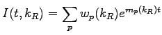
where P$^{i}$(r,t) is the probability to find an atom at an arbitrary site if the atom was at the time t=0 and position r=0 at a site with symmetry $i$, P$^{j}_{i}$(r,t) is the probability to find an atom on a certain site with symmetry i if the atom was at the time t=0 and position r=0 at a site with symmetry j. As sketched in figure the next step is the Fourier transform in space which leads immediately to the intermediate-scattering function I(t,k$_R$).

$$I(t,k_{R})=\frac{1}{2\pi}\int^{\infty}_{-\infty} G(t, k_{R}) e^{i\omega r} dr$$ (62)

This definition allows to rewrite the set of differential equations into a set of equations for the intermediate-scattering function

$$\frac{\partial I_{i}(t,r)}{\partial t}=\sum _{j,k,j\neq k}\bigg{(... ...i}(t,r+l_{ijk})}{n_{ji}\tau_{ji}} -\frac{ I_{i}(t,r)}{n_{ij}\tau_{ij}} \bigg{)}$$ (63)

or written in a matrix form

$$\frac{\partial}{\partial t} I_{i}(t,r)=A \cdot I,$$ (64)

with

$$A_{ij}=\frac{1}{n_{ij}\tau_{ij}}\sum_{k}e^{k_{R}l_{ijk}}$$

$$A_{ii}=-\sum_{j=1,j\neq i}^{m}\frac{1}{n_{ij}\tau_{ij}}.$$ (65)

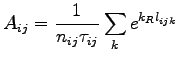
The matrix A is called the jump matrix and contains all information about the jump-diffusion mechanism (jump frequencies and jump vectors). The jump matrix A can be transformed into a Hermitian matrix B using the following transformation

$$B=T\cdot A\cdot T^{-1}$$ (66)

with the transformation matrix T

$$T_{ij}=\delta_{ij}\sqrt{\frac{1}{c_{ij}}}$$ (67)

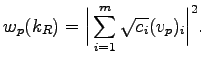
The set of differential equations can be solved now calculating the eigenvalues $m_{p}$ and eigenvectors $v_{p}$ of the matrix B. The solution is the sum

$$I(t,k_{R})=\sum_{p}w_{p}(k_{R})e^{m_{p}(k_{R})t}$$ (68)

with weights $w{_p}$(k$_R$)defined by the eigenvectors $v{_p}$ of the matrix B

$$w_{p}(k_{R})=\bigg{\vert}\sum_{i=1}^{m}\sqrt{c_{i}}(v_{p})_{i} \bigg{\vert}^{2}.$$ (69)

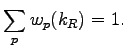
The weights have to fulfil the condition

$$\sum_{p}w_{p}(k_{R})=1.$$ (70)

From equation it is clear that the general shape of the intermediate-scattering function I(t,k$_{R}$) is a sum of $p$ exponential functions, each sublattice resulting in one exponential decay, with the decay rate corresponding to the eigenvalues $m_{p}$(k$_{R}$) of the matrix B. The eigenvalues are a function of the outgoing wave vector k$_R$ and of the jump frequency 1/$\tau_{ij}$ (equation ). Generally a higher jump frequency will result in a faster decay of the intermediate-scattering function. This faster decay is usually called ``accelerated decay''.
The crucial point now is to use the result of the calculation in this chapter as an input into the ``recipe'' for the calculation of the time spectrum of a layer or multilayer (equations and respectively). The idea was to use the frequency dependence of the refractive index and follow the exact Par

$$I(\omega,k_{R})=\frac{1}{\pi}\sum_{p}\frac{\frac{\Gamma _{0}+\Gam... ...ga-\omega_{0})^{2}+\bigg{(}\frac{\Gamma _{0}+\Gamma _{p}} {2\hbar}\bigg{)}^{2}}$$ (71)

with

$$\Gamma (k_{R})_{p}=-2\hbar m_{p}(k_{R})$$ (72)

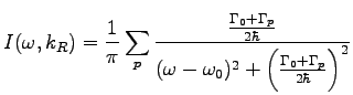
In analogy to the sum of exponentials in equations , each sublattice results in the energy domain in an Lorentzian line with the line width $\Gamma$(k$_{_R}$)=$\Gamma_{0}$+$\Gamma_{p}$(k$_{_R}$) defined in equation . The line width $\Gamma$ is the most important input parameter for the calculation of the the jump-diffusion mechanism. It contains the information about the jump frequencies and jump vectors. The resulting $\Gamma$(k$_R$) can be inserted into the equation for the refractive index and used to calculate the total reflectivity and the intermediate-scattering function.