In the previous sections only unsplit resonances of a nucleus have been discussed. However, a nucleus interacts with the surrounding electronic density ![]() . These interactions are called hyperfine interactions and result into a splitting of the excited and/or ground state into more states. Each allowed transition between these states is manifested by a Lorentzian line in energy domain. In this section the quadrupole interaction, which is important for the understanding of further details, will be discussed.
Assumed is a nucleus with a nuclear density
. These interactions are called hyperfine interactions and result into a splitting of the excited and/or ground state into more states. Each allowed transition between these states is manifested by a Lorentzian line in energy domain. In this section the quadrupole interaction, which is important for the understanding of further details, will be discussed.
Assumed is a nucleus with a nuclear density ![]() surrounded by an electronic charge producing the potential
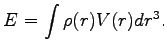
surrounded by an electronic charge producing the potential ![]() . The interaction energy between the nucleus and the potential is
. The interaction energy between the nucleus and the potential is
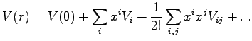
The potential can be written as a Taylor expansion series around the origin
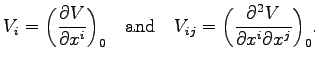
with
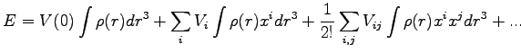
Inserting the Taylor series into equation ![[*]](crossref.png) the interaction energy can be rewritten as
the interaction energy can be rewritten as
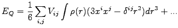
The first term refers to the electrostatic energy of a point like nucleus. The second term corresponds to the dipole interaction of the nucleus and disappears in the case of a spherical nuclear charge distribution. The third term is the most interesting for this work. It is the quadrupole interaction. It generates multiple line spectra and can deliver a lot of information about the coordination and kind of the nearest neighbours of the investigated nucleus. The tensor ![]() , called the electric field gradient (EFG), is traceless if the potential is created by charges in the surrounding of the nucleus.
, called the electric field gradient (EFG), is traceless if the potential is created by charges in the surrounding of the nucleus.
Due to this property the quadrupole interaction can be written as
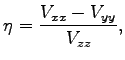
Defining the asymmetry parameter
only two independent parameters are necessary to describe the electric field gradient completely. Usually the convention
![]() is used to ensure that
is used to ensure that
![]() .
.
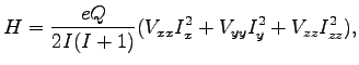
The Hamiltonian describing the quadrupole interaction is
where ![]() are the conventional spin operators. In the simplest case the EFG tensor
are the conventional spin operators. In the simplest case the EFG tensor ![]() has an axial symmetry and the asymmetry parameter
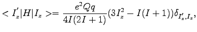
has an axial symmetry and the asymmetry parameter ![]() =0. In this case the matrix elements for a nucleus with the spin
=0. In this case the matrix elements for a nucleus with the spin ![]() are given by
are given by
or in other words the ground and excited states are split into different levels corresponding to ![]() and
and ![]() . For the investigated Mössbauer nucleus, i.e.
. For the investigated Mössbauer nucleus, i.e. ![]() Fe, the ground state with the spin I=1/2 results into one unsplit level and the excited state with spin I=3/2 splits into two levels with the energies
Fe, the ground state with the spin I=1/2 results into one unsplit level and the excited state with spin I=3/2 splits into two levels with the energies
According to the equation the classical Mössbauer spectrum will contain two Lorentzian lines with the positions corresponding to the ![]() of the Hamiltonian
of the Hamiltonian
as shown in figure on the left side.
![\includegraphics[width=0.8\textwidth]{pics/quantum_beats}](img212.png)
|
The time response is changing drastically compared to the simple exponential shape in the thin sample limit. Both waves re-emitted by the Mössbauer atom with slightly different frequencies interfere in the detector and produce quantum beats. A simulated Mössbauer spectrum compared with the corresponding NRS spectrum is shown in figure . Please note that a decrease of the interaction energy decreases the splitting of the absorption lines but increases the period of the quantum beats. These period of the quantum beat can be roughly connected with the splitting in the energy using the simple approximation
i.e. the smaller the quadrupole splitting the larger the quantum beat period.