Mössbauer effect

The discovery of the Mössbauer effect, i.e. of the recoilless emission and absorption of gamma radiation by atomic nuclei by R. L. Mößbauer 1957 (figure ) [25] made the evolution of resonance spectroscopy with low energy gamma radiation possible. As usual for each resonant spectroscopy, the basis is a resonant excitation. In this case a photon emitted during an energy transition (Mössbauer spectroscopy [26,27]) or during an acceleration of an electron [28] with a well defined energy $\hbar\omega$, excites a nucleus into a high energy state. 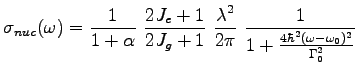The nucleus decays then with characteristic lifetime $\tau_{0}$ into the ground state and re-emits a photon with exactly the same energy. From the resonant nature of the effect it is clear that the cross section of a resonant atom depends very strongly on the frequency of the photon $\omega$

$$\sigma_{nuc}(\omega)=\frac{1}{1+\alpha} \ \frac{2J_{e}+1}{2J_{g}+... ...}}{2\pi} \ \frac{1}{1+\frac{4\hbar^{2}(\omega-\omega_{0})^{2}}{\Gamma_{0}^{2}}}$$ (33)

where $J_{e}$ and $J_{g}$ are the spins of the resonant nucleus in the excited and ground state, $\omega_{0}$ is the resonant frequency, $\lambda$ is the wavelength of the radiation, $\Gamma_{0}$ is the natural line width, which is connected with the lifetime of the resonant nucleus $\tau_{0}$ by the uncertainty relation $\Gamma_{0}\tau_{0}=h$ and $\alpha$ is the internal conversion coefficient (and not the incident angle), which describes the probability for re-emission of a photon and not, e.g., of a conversion electron ($\alpha$ = 8.2 for the 14.4 $keV$ transition in $^{57}$Fe). It is important to note at this point that the excited state is not split into multiple states by hyperfine interaction (e.g. Zeeman effect) and effects of polarisation of the used radiation are not taken into account.

Figure: Nobel prize winner R. L. Mößbauer (right) with the author of this work (left) on the International Conference on the Applications of the Mössbauer Effect (ICAME) 1999 in Garmisch-Partenkirchen, Germany.

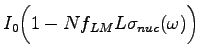
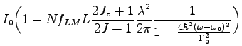
The energy of the incident radiation in a typical Mössbauer experiment is modulated by a Doppler drive. This allows the experimentator to scan the energy states of the resonant nuclei in the sample mounted in a furnace . The transmitted radiation is detected in a detector as a function of the velocity of the Doppler drive (energy). The intensity $I(\omega)$ measured in the detector is in the limit of a thin sample

$$I(\omega) = I_{0}\bigg{(}1-Nf_{LM}L\sigma_{nuc}(\omega)\bigg{)}$$

$$= I_{0}\bigg{(}1-Nf_{LM}L\frac{2J_{e}+1}{2J_{}+1}\frac{\lambda^{2}}{2\pi}\frac{1}{1+\frac{4\hbar^{2}(\omega-\omega_{0})^{2}}{\Gamma_{0}^{2}}}\bigg{)}$$ (34)

where N is the atomic density of Mössbauer nuclei in the sample, $f_{LM}$ is the Lamb-Mössbauer factor, L is the thickness of the sample and I$_{0}$ is the flux of the source.

Figure: Typical setup for a Mössbauer experiment: The incident radiation, modulated by a Doppler drive, scans the energy states of the resonant nuclei in the sample mounted in the furnace. The transmitted radiation is detected in the detector as a function of the velocity of the Doppler drive (energy).